A transparent photoelastic polymer containing a single hole of \(500\mu m\) is loaded under tensile stress. The same experiment is done again using Digital Image Correlation (DIC) as an analysis method this time. The contour plot shown in the DIC experiment are percentiles of \( \epsilon_1 \) - \( \epsilon_2 \), where \( \epsilon_{1} \) is the deformation in the first principal direction and \(\epsilon_2\) the deformation in the second principal direction. The number of photoelastic fringes passing through a material point on the specimen’s surface is also proportional to \( \epsilon_1- \epsilon_2 \), allowing a qualitative comparison of both methods by looking at:

• The fringes concentration
• The number of fringes passing through a single material point and their direciton

This video compares both methods.

Both specimens’ dimensions were chosen according to the ASTM D632 Type V. Test speed: \(0.1mm/min\)

It is possible to see that the photoelastic specimen firstly reveals large fringes going through the whole specimen from left to right, that is probably because the specimen is experimenting torsion, due to the fact it was not perfectly straight between the grips. Once the whole specimen emits an almost uniform color (second 40), 6 petal fringes (circular) are cricling the hole.

Experiments done in collaboration with Rolland Delorme, at Ecole Polytechnique Montreal during November 2015.

If you liked this post, you can share it with your followers or follow me on Twitter!

When capturing images from a lab camera, you might find yourself with a bunch of .tiff images.

The first thing you will need is the ImageMagick package for Ubuntu. You can get it using:

sudo apt-get install imagemagick

This package contains a very convenient convert function, it can be used to convert a .tiff image into a .png while keeping transparency using:

convert inputfile.tiff -transparent white outputfile.png

You can then use this command to recursively treat any file in the folder with a simple grep and some batch scripting:

    #!/bin/sh
    for file in `ls | grep tif`
    do
        convert "$file" -transparent white "${file}.png"
        echo "writing ${file}.png"
    done

To use it, you simply need to put a bunch of .tiff files in the same folder, and execute the script. If your files are recorded as .tif and not .tiff, you will need to change it in the second line of the script.

Final tip: If any other file in the folder (it can be the script itself) contains the letters T-I-F-F in this order, it will be transformed into a .png even if it is a text file.

Source, more details: http://ospublish.constantvzw.org/blog/tools/convert-tiff-to-transparent-png

If you liked this post, you can share it with your followers or follow me on Twitter!

Implementing nice looking plots in a \(\LaTeX\) document was harder than expected. I use R (through Rstudio) combined with ggplot2 (Grammar of Graphics plot) to plot my data and wanted a convenient way to insert my plots into Latex documents. I use something similar with Inkscape. It automatically sets the right font, properly writes Latex symbols and respects the proper font sizes.

The best solution I found is using the tikzDevice package for R and the tikz (available in the pgf package) package from LaTeX. TikZ plots will consist of vectors that will directly be coded into the LaTeX document so that there is no loss in image quality. First you need to install tikzDevice in R through install.packages("tikzDevice"). For the following example to work, you will also need to install ggplot2. Once you have both R packages, you can use this Rscript as an example:

	library(tikzDevice)
	library(ggplot2)
	#For some reason, Rstudio needs to know the time zone...
	options(tz="CA")
	#Dummy data for the plot
	y <- exp(seq(1,10,.1))
	x <- 1:length(y)
	data <- data.frame(x = x, y = y)

	#Create a .tex file that will contain your plot as vectors
	#You need to set the size of your plot here, if you do it in LaTeX, font consistency with the rest of the document will be lost
	tikz(file = "plot_test.tex", width = 5, height = 5)
	#Simple plot of the dummy data using LaTeX elements
	plot <- ggplot(data, aes(x = x, y = y)) + 
		geom_line() +
		#Space does not appear after Latex
		ggtitle( paste("Fancy \\LaTeX ", "\\hspace{0.01cm} title")) +
		labs( x = "$x$ = Time", y = "$\\Phi$ = Innovation output") +
		theme_bw()
	#This line is only necessary if you want to preview the plot right after compiling
	print(plot)
	#Necessary to close or the tikxDevice .tex file will not be written
	dev.off()

The output provided by this script in R looks like this:

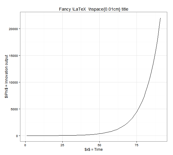
As you can see, the LaTeX codes are clearly visible. The font is R’s default font for now. If you check the folder where you sourced your file, you will find a test.tex file(you can check its content for this specific case by clicking on it) which contains the plot information as vectors. Every line, word or symbol is included as latex instructions in this .tex file. You should now create a .tex (any name will do) in the same folder your plot_test.tex file is in and use this simple LaTeX code to implement the image in it:

	\documentclass{article}
	%The package tikz is available in pgf
	\usepackage{tikz}
	\begin{document}

	\begin{figure}
		%Do not try to scale figure in .tex or you loose font size consistency
	    	\centering
		%The code to input the plot is extremely simple
		\input{plot_test.tex}
		%Captions and Labels can be used since this is a figure environment
		\caption{Sample output from tikzDevice}
		\label{plot:test}
	\end{figure}
	\end{document}

The result should look like this. As you can see, LaTeX symbols are now properly written, the font is also similar to the rest of the document and the plot can be inserted in your LaTeX document !

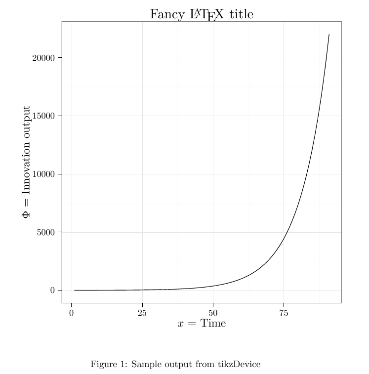
A problem you might still have: the font size of the plot title and axis legend and their positions. You can easily modify the sizes using the rel() function to scale the font size of each element. To modify the position of the axis legends or title plot, you can use the vjust and hjust parameters for vertical and horizontal positioning. R will not prepare your plot for the LaTeX font and sizes, so you will probably need to move the title and axis titles or they will probably touch the plot itsel at some point (visible in the previous LaTeX plot). To correct it, use something similar to this:

        plot + theme(plot.title = element_text(size = rel(1), vjust = 0), 
        axis.title = element_text(size = rel(0.8)),
        axis.title.y = element_text( vjust=2 ),
        axis.title.x = element_text( vjust=-0.5 ))

If you liked this post, you can share it with your followers or follow me on Twitter!

After the Windows 10 update, Miktex refused to download new packages and kept signaling a Windows API Error 2. The worst part was that the uninstall file for Miktex was nowhere to be found, which made it impossible to properly uninstall it using Windows Program manager. On the machine’s Admin account, Miktex was not even reported in the Program manager anymore.

A simple and efficient fix that worked for me is to rename you current Miktex folder Miktex_old, install Miktex where the old install was and simply delete the Miktex_old folder, and that’s it !

This trick might also repair some of the other numerous bugs Miktex meets on a Windows system (especially 64bits).

If you liked this post, you can share it with your followers or follow me on Twitter!

You can easily check if someone is connected to a Wifi network using a simple function provided in the Network MAP package. Nmap is a security package designed to discover hosts, services and machines on a network.

Setting up

First, you need to install Nmap and its python wrapper:

	sudo apt-get install nmap
	sudo pip install python-nmap

Use it

You can either use the python console to perform unique scans or script your scans to perform them on a regular basis. You will need to be root in order to use nmap.

#First, you need a Postscanner object that will be used to do the scan
nm = nmap.PortScanner()
#You can then do a scan of all the IPV4 addresses provided by the network you are connected to
nm.scan(hosts = '192.168.1.0/24', arguments = '-sn')

The 3 first numbers of the IP address (192.168.1) used as hosts might need to be changed depending of the network. Check the IP address of a machine connected to that same network to know which hosts you should scan. You can then check the all_hosts() function attached to the PortScanner object which provides a list containing information about each IP address available in the network. For each element, you can check several values such as the MAC address.

	for host in nm.all_hosts():
		#If the status of an IP address is not down, print it
		if nm[host]['status']['state'] != "down":
			print "STATUS:", nm[host]['status']['state']
			#Print the MAC address
			try:
				print "MAC ADDRESS:", nm[host]['addresses']['mac']
			except:
				mac = 'unknown'

For some devices, the MAC address is not openly displayed.

Implementation

The best way to use this is to set up a Raspberry Pi running a script with a Cron job regularly scanning your network and notifying you through an intranet webpage, mail or SMS if any interesting event happens. To do so, you need to know the MAC address of your roommates’ smartphones or laptops. You can also use it for network discovery. You will quickly notice that you can attach MAC addresses to people by performing Nmap is a much more powerful tool than what is presented here. This is just a fun trick that can be used with roommates to play an intro music when they get home for example.

Now that I know that anyone can get my MAC addresses by performing simple scans when I am connected to a WiFi network and when I am not, what I would like to know is how can one be protected from such attempts? Is it possible to voluntarily hide your MAC address from the netowrk?

PS: Check NMap’s presence in blockbuster movies

If you liked this post, you can share it with your followers or follow me on Twitter!